LeNet 5 Architecture Explained

This is the fourth blog from my Computer Vision series. As we are moving forward after learning all the basics of the Convolution Neural Networks we will be studying various CNN Architectures that have been developed during the enhancement of AI Technology.

If you haven’t checked out my previous blogs on this topic I would recommend checking them out:

Why Convolutions?
Understanding Convolution Neural Networks Part 1 and Part 2

LeNet 5 architecture is the ‘Hello World’ in the domain of Convolution Neural Networks. The backpropagation rule was first applied to all reasonable applications in 1989 by Yann LeCun and colleagues at Bell Labs. They also argued that by imposing limitations from the tasks domain, network generalization’s flexibility could be significantly strengthened. LeCun established that single-layer networks do tend to exhibit weak generalisation skills by explaining a modest handwritten digit identification anomaly in another publication within the same year, even supposing the problem is linearly separable. A multi-layered, unnatural network may function exceptionally well once an anomaly is eliminated using invariant feature detectors. He thought that these findings proved that reducing the number of free parameters in the neural network could improve its ability to generalise.

💡 What is LeNet 5?

LeNet is a convolutional neural network that Yann LeCun introduced in 1989. LeNet is a common term for LeNet-5, a simple convolutional neural network.

The LeNet-5 signifies CNN’s emergence and outlines its core components. However, it was not popular at the time due to a lack of hardware, especially GPU (Graphics Process Unit, a specialised electronic circuit designed to change memory to accelerate the creation of images during a buffer intended for output to a show device) and alternative algorithms, like SVM, which could perform effects similar to or even better than those of the LeNet.

📌 Features of LeNet-5

Every convolutional layer includes three parts: convolution, pooling, and nonlinear activation functions
Using convolution to extract spatial features (Convolution was called receptive fields originally)
The average pooling layer is used for subsampling.
‘tanh’ is used as the activation function
Using Multi-Layered Perceptron or Fully Connected Layers as the last classifier
The sparse connection between layers reduces the complexity of computation

💡 Architecture

The LeNet-5 CNN architecture has seven layers. Three convolutional layers, two subsampling layers, and two fully linked layers make up the layer composition.

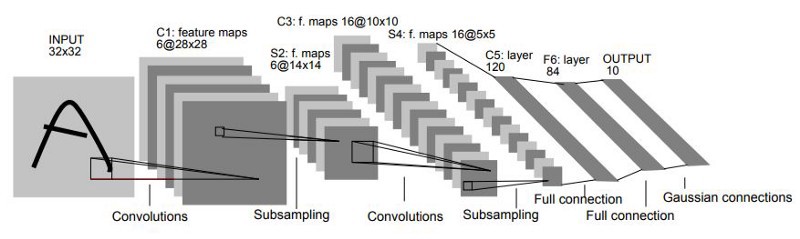
🖼 LeNet-5 Architecture

📌 First Layer

A 32x32 grayscale image serves as the input for LeNet-5 and is processed by the first convolutional layer comprising six feature maps or filters with a stride of one. From 32x32x1 to 28x28x6, the image’s dimensions shift.

🖼 First Layer

📌 Second Layer

Then, using a filter size of 22 and a stride of 2, the LeNet-5 adds an average pooling layer or sub-sampling layer. 14x14x6 will be the final image’s reduced size.

🖼 Second Layer

📌 Third Layer

A second convolutional layer with 16 feature maps of size 55 and a stride of 1 is then present. Only 10 of the 16 feature maps in this layer are linked to the six feature maps in the layer below, as can be seen in the illustration below.

The primary goal is to disrupt the network’s symmetry while maintaining a manageable number of connections. Because of this, there are 1516 training parameters instead of 2400 in these layers, and similarly, there are 151600 connections instead of 240000.

🖼 Third Layer

📌 Fourth Layer

With a filter size of 22 and a stride of 2, the fourth layer (S4) is once more an average pooling layer. The output will be decreased to 5x5x16 because this layer is identical to the second layer (S2) but has 16 feature maps.

🖼 Fourth Layer

📌 Fifth Layer

With 120 feature maps, each measuring 1 x 1, the fifth layer (C5) is a fully connected convolutional layer. All 400 nodes (5x5x16) in layer four, S4, are connected to each of the 120 units in C5’s 120 units.

🖼 Fifth Layer

📌 Sixth Layer

A fully connected layer (F6) with 84 units makes up the sixth layer.

🖼 Sixth Layer

📌 Output Layer

The SoftMax output layer, which has 10 potential values and corresponds to the digits 0 to 9, is the last layer.

🖼 Output Layer

💡 Summary of LeNet-5 Architecture

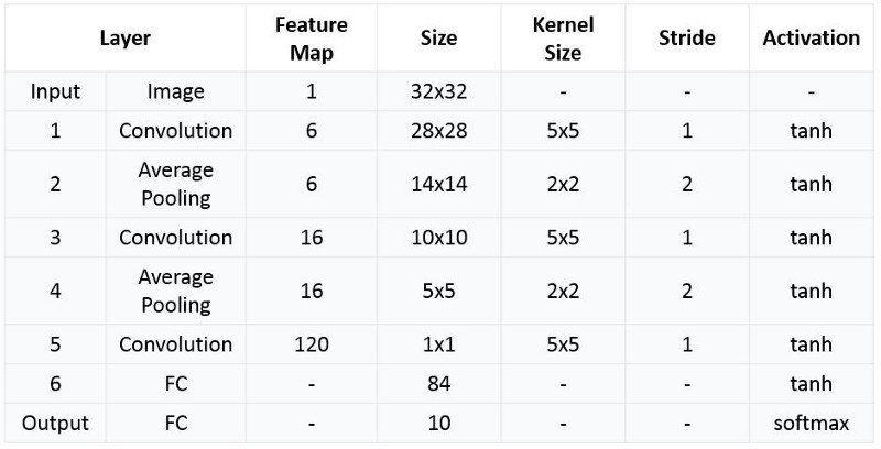
🖼 Summarized table for LeNet 5 Architecture

💡 Implementation

We will be implementing the LeNet-5 Architecture on the MNIST Dataset because MNIST Dataset has images of 28x28 size which have characters are written that will help to show the better implementation of the architecture.

You can study more about the MNIST Dataset and can download the dataset from here — MNIST Dataset.

Although, MNIST Dataset is one of the practice datasets that are available in the TensorFlow library just for implementing and practising.

📌 Download and Load the Dataset

import matplotlib.pyplot as plt
import tensorflow as tf
import numpy as np

mnist = tf.keras.datasets.mnist
(x_train, y_train), (x_test, y_test) = mnist.load_data()

📌 Pre-processing and Normalizing the Data

rows, cols = 28, 28

# Reshape the data into a 4D Array
x_train = x_train.reshape(x_train.shape[0], rows, cols, 1)
x_test = x_test.reshape(x_test.shape[0], rows, cols, 1)

input_shape = (rows,cols,1) 

# Set type as float32 and normalize the values to [0,1]
x_train = x_train.astype('float32')
x_test = x_test.astype('float32')
x_train = x_train / 255.0
x_test = x_test / 255.0

# Transform labels to one hot encoding
y_train = tf.keras.utils.to_categorical(y_train, 10)
y_test = tf.keras.utils.to_categorical(y_test, 10)

📌 Define LeNet-5 Model

def build_lenet(input_shape):
  # Define Sequential Model
  model = tf.keras.Sequential()

  # C1 Convolution Layer
  model.add(tf.keras.layers.Conv2D(filters=6, strides=(1,1), kernel_size=(5,5), activation='tanh', input_shape=input_shape))

  # S2 SubSampling Layer
  model.add(tf.keras.layers.AveragePooling2D(pool_size=(2,2), strides=(2,2)))

  # C3 Convolution Layer
  model.add(tf.keras.layers.Conv2D(filters=6, strides=(1,1), kernel_size=(5,5), activation='tanh'))

  # S4 SubSampling Layer
  model.add(tf.keras.layers.AveragePooling2D(pool_size=(2,2), strides=(2,2)))

  # C5 Fully Connected Layer
  model.add(tf.keras.layers.Dense(units=120, activation='tanh'))

  # Flatten the output so that we can connect it with the fully connected layers by converting it into a 1D Array
  model.add(tf.keras.layers.Flatten())

  # FC6 Fully Connected Layers
  model.add(tf.keras.layers.Dense(units=84, activation='tanh'))

  # Output Layer
  model.add(tf.keras.layers.Dense(units=10, activation='softmax'))

  # Compile the Model
  model.compile(loss='categorical_crossentropy', optimizer=tf.keras.optimizers.SGD(lr=0.1, momentum=0.0, decay=0.0), metrics=['accuracy'])

  return model

Create a new instance of a model object using sequential model API. Then add layers to the neural network as per the LeNet-5 architecture discussed earlier. Finally, compile the model with the ‘categorical_crossentropy’ loss function and ‘SGD’ cost optimization algorithm. When compiling the model, add metrics=[‘accuracy’] as one of the parameters to calculate the accuracy of the model.

It is important to highlight that each image in the MNIST data set has a size of 28 X 28 pixels so we will use the same dimensions for LeNet-5 input instead of 32 X 32 pixels.

📌 Evaluate the Model and Visualize the process

We can train the model by calling the model.fit function and pass in the training data, the expected output, the number of epochs, and batch size. Additionally, Keras provides a facility to evaluate the loss and accuracy at the end of each epoch. For this purpose, we can split the training data using the ‘validation_split’ argument or use another dataset using the ‘validation_data’ argument. We will use our training dataset to evaluate the loss and accuracy after every epoch.

We can test the model by calling model.evaluate and passing in the testing data set and the expected output.

We will visualize the training process by plotting the training accuracy and loss after each epoch.

lenet = build_lenet(input_shape)

# We will be allowing 10 itterations to happen
epochs = 10
history = lenet.fit(x_train, y_train, epochs=epochs,batch_size=128, verbose=1)

# Check Accuracy of the Model
loss ,acc= lenet.evaluate(x_test, y_test)
print('Accuracy : ', acc)

x_train = x_train.reshape(x_train.shape[0], 28,28)
print('Training Data', x_train.shape, y_train.shape)
x_test = x_test.reshape(x_test.shape[0], 28,28)
print('Test Data', x_test.shape, y_test.shape)

# Plot the Image
image_index = 8888
plt.imshow(x_test[image_index].reshape(28,28), cmap='Greys')

# Make Prediction
pred = lenet.predict(x_test[image_index].reshape(1, rows, cols, 1 ))
print(pred.argmax())

'''
Epoch 1/10
469/469 [==============================] - 2s 3ms/step - loss: 0.4411 - accuracy: 0.8755
Epoch 2/10
469/469 [==============================] - 2s 3ms/step - loss: 0.1870 - accuracy: 0.9447
Epoch 3/10
469/469 [==============================] - 2s 3ms/step - loss: 0.1367 - accuracy: 0.9589
Epoch 4/10
469/469 [==============================] - 2s 3ms/step - loss: 0.1103 - accuracy: 0.9666
Epoch 5/10
469/469 [==============================] - 2s 3ms/step - loss: 0.0931 - accuracy: 0.9723
Epoch 6/10
469/469 [==============================] - 2s 3ms/step - loss: 0.0811 - accuracy: 0.9750
Epoch 7/10
469/469 [==============================] - 2s 4ms/step - loss: 0.0722 - accuracy: 0.9781
Epoch 8/10
469/469 [==============================] - 2s 3ms/step - loss: 0.0654 - accuracy: 0.9794
Epoch 9/10
469/469 [==============================] - 2s 3ms/step - loss: 0.0606 - accuracy: 0.9818
Epoch 10/10
469/469 [==============================] - 2s 3ms/step - loss: 0.0560 - accuracy: 0.9827
313/313 [==============================] - 1s 2ms/step - loss: 0.0543 - accuracy: 0.9808
Accuracy :  0.9807999730110168
Training Data (60000, 28, 28) (60000, 10)
Test Data (10000, 28, 28) (10000, 10)
6
'''

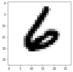
🖼 Output Visualization

Siddhesh's Blog