Understanding Convolutional Neural Networks (Part 2)

Master's student @Trinity College Dublin | Loves solving complex problems through intelligent systems | Exploring jobs in tech
🖼 Visual Representation of CNN
If you have not yet read the preceding part of this blog, go here to do so so that you can better comprehend the topics presented in this blog. — Understanding Convolution Neural Networks (Part 1)
We studied a few foundations underlying the working of Convolution Neural Networks in the last blog, such as padding, stride, kernels, filters, and so on. Let’s go over a few more CNN ideas and see how the Convolution Neural Network works in practice with TensorFlow and Keras.
📌 Receptive Fields
Formally, it is the region in the input space that a particular CNN’s feature is affected by. More informally, it is the part of a tensor that after convolution results in a feature. So basically, it gives us an idea of where we’re getting our results from as data flows through the layers of the network.
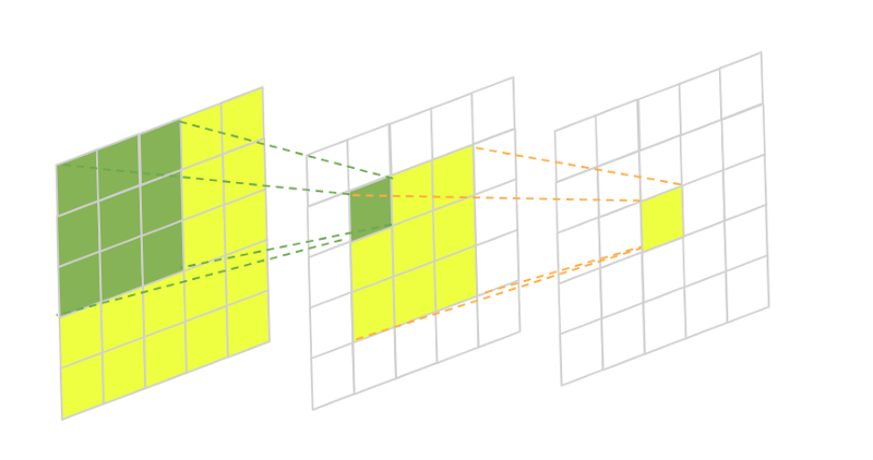
🖼 Receptive Field Intuition
In this image, we have a two-layered fully-convolutional neural network with a 3×3 kernel in each layer. The green area marks the receptive field of one pixel in the second layer and the yellow area marks the receptive field of one pixel in the third final layer.
Usually, we’re mostly interested in the size of the receptive field in our initial input to understand how much area the CNN covers from it. This is essential in many computer vision tasks. Take, for example, image segmentation. The network takes an input image and predicts the class label of every pixel building a semantic label map in the process. If the network can’t take into account enough surrounding pixels when doing its predictions some larger objects might be left with incomplete boundaries.
The same thing applies to object detection. If the convolutional neural network doesn’t have a large enough receptive field some of the larger objects on the image might be left undetected.
💡 Local Receptive Field
All input Neurons are just pixel intensities of an input image and many hidden Neurons in the first hidden layer.
If Neuron is connected to only a small region of the input layer neurons then that region in the input image is called the Local receptive field for the hidden neuron.
Each connection with the local receptive field has weight, which will learn during the training of our model.
Each hidden Neuron will learn a particular local receptive field.
🖼 Local Receptive Field
You can study more deeply about Local Receptive Field in this blog by Richmond Alake (This is a premium blog, you need to have a Medium account or Medium Premium account subscription to read the blog.)— Local Receptive Field
💡 Global Receptive Field
A Global Receptive Field is nothing but the original size of the image which is to be reduced during the process of convolution. For Example, if there is an image i1 of size 7x7, and we use a filter k1 of size 3x3 on i1 to produce another image i2 which is of size 5x5, and again apply the filter k2 with the same size of 3x3 to produce final image i3. Here the local receptive field for i3 will be the size of i2 i.e. 5x5 but the global receptive field of the i3 will be the original image size i.e. i1 7x7.
📌 Output Dimensionality Size
Imagine, there is an image of size 200x200, how many convolutional layers would require to make that 200x200 image into a 1x1 image using a 3x3 kernel? It will take a lot of layers as well as a lot of computation power to train such kind of data because we know that after every convolution of an image by a 3x3 kernel the size just gets reduced by 2x2, i.e. if a 200x200 image is in the first layer getting convoluted by 3x3 kernel then the output would be 198x198, then 196x196, 194x194 and so on till it reaches 1x1. Always remember that a normal CNN architecture should have 5–15 layers, max to max 16–32, although it depends upon the resolution of the image. This issue of reducing the layers is generally solved by adding a Max-Pooling layer.
📌 Max Pooling
Max Pooling is a feature commonly imbibed into Convolutional Neural Network (CNN) architectures. The main idea behind a pooling layer is to “accumulate” features from maps generated by convolving a filter over an image. Formally, its function is to progressively reduce the spatial size of the representation to reduce the number of parameters and computations in the network. The most common form of pooling is max pooling.

🖼 Max Pooling Concept
Max pooling is done in part to help over-fitting by providing an abstracted form of the representation. As well, it reduces the computational cost by reducing the number of parameters to learn and provides basic translation invariance to the internal representation. Max pooling is done by applying a max filter to (usually) non-overlapping sub-regions of the initial representation. The other forms of pooling are average and min. In Max-pooling we generally refer to filters or kernels as a mask because they extract and encapsulate more data as compared to that the filters and kernels.
import keras
from keras.models import Sequential
from keras.layers import Activation
from keras.layers.core import Dense, Flatten
from keras.layers.convolutional import *
from keras.layers.pooling import *

model_valid = Sequential([
    Dense(16, input_shape=(20,20,3), activation='relu'),
    Conv2D(32, kernel_size=(3,3), activation='relu', padding='same'),
    MaxPooling2D(pool_size=(2, 2), strides=2, padding='valid'),
    Conv2D(64, kernel_size=(5,5), activation='relu', padding='same'),
    Flatten(),
    Dense(2, activation='softmax')
])
🌀 Practice Intuition on MNIST Dataset
📌 Load MNIST Dataset
MNIST is one of the most famous datasets in the field of machine learning.
It has 70,000 images of hand-written digits
Very straightforward to download
Images dimensions are 28x28
Grayscale images
from tensorflow.keras.datasets import mnist

# use Keras to import pre-shuffled MNIST database
(X_train, y_train), (X_test, y_test) = mnist.load_data()

print("The MNIST database has a training set of %d examples." % len(X_train))
print("The MNIST database has a test set of %d examples." % len(X_test))
📌 Visualize first six training images
import matplotlib.pyplot as plt
%matplotlib inline
import matplotlib.cm as cm
import numpy as np

# plot first six training images
fig = plt.figure(figsize=(20,20))
for i in range(6):
    ax = fig.add_subplot(1, 6, i+1, xticks=[], yticks=[])
    ax.imshow(X_train[i], cmap='gray')
    ax.set_title(str(y_train[i]))

📌 View the Image in more detail
def visualize_input(img, ax):
    ax.imshow(img, cmap='gray')
    width, height = img.shape
    thresh = img.max()/2.5
    for x in range(width):
        for y in range(height):
            ax.annotate(str(round(img[x][y],2)), xy=(y,x),
                        horizontalalignment='center',
                        verticalalignment='center',
                        color='white' if img[x][y]<thresh else 'black')

fig = plt.figure(figsize = (12,12))
ax = fig.add_subplot(111)
visualize_input(X_train[0], ax)

📌 Pre-process Images and Labels
Pre-Process images by rescaling i.e. dividing every pixel in every image by 255 and pre-process labels by encoding categorical integer labels using the one-hot encoding scheme.
# rescale to have values within 0 - 1 range [0,255] --> [0,1]
X_train = X_train.astype('float32')/255
X_test = X_test.astype('float32')/255

print('X_train shape:', X_train.shape)
print(X_train.shape[0], 'train samples')
print(X_test.shape[0], 'test samples')

from keras.utils import np_utils

num_classes = 10
# print first ten (integer-valued) training labels
print('Integer-valued labels:')
print(y_train[:10])

# one-hot encode the labels
# convert class vectors to binary class matrices
y_train = np_utils.to_categorical(y_train, num_classes)
y_test = np_utils.to_categorical(y_test, num_classes)

# print first ten (one-hot) training labels
print('One-hot labels:')
print(y_train[:10])
📌 Reshape data to fit our CNN
# input image dimensions 28x28 pixel images.
img_rows, img_cols = 28, 28

X_train = X_train.reshape(X_train.shape[0], img_rows, img_cols, 1)
X_test = X_test.reshape(X_test.shape[0], img_rows, img_cols, 1)
input_shape = (img_rows, img_cols, 1)

print('input_shape: ', input_shape)
print('x_train shape:', X_train.shape)
📌 Define Model Architecture
You must pass the following arguments:
filters — The number of filters.
kernel_size — Number specifying both the height and width of the (square) convolution window.
There are some additional, optional arguments that you might like to tune:
strides — The stride of the convolution. If you don’t specify anything, strides are set to 1.
padding — One of ‘valid’ or ‘same’. If you don’t specify anything, padding is set to ‘valid’.
activation — Typically ‘relu’. If you don’t specify anything, no activation is applied. You are strongly encouraged to add a ReLU activation function to every convolutional layer in your networks.
💡 Things to remember
Always add a ReLU activation function to the Conv2D layers in your CNN. Except for the final layer in the network, Dense layers should also have a ReLU activation function.
When constructing a network for classification, the final layer in the network should be a Dense layer with a SoftMax activation function. The number of nodes in the final layer should equal the total number of classes in the dataset.
from tensorflow.keras.models import Sequential
from tensorflow.keras.layers import Conv2D, MaxPooling2D, Flatten, Dense, Dropout, GlobalAveragePooling2D

# build the model object
model = Sequential()

# CONV_1: add CONV layer with RELU activation and depth = 32 kernels
model.add(Conv2D(32, kernel_size=(3, 3), padding='same',activation='relu',input_shape=(28,28,1)))
# POOL_1: downsample the image to choose the best features
model.add(MaxPooling2D(pool_size=(2, 2)))

# CONV_2: here we increase the depth to 64
model.add(Conv2D(64, (3, 3),padding='same', activation='relu'))
# POOL_2: more downsampling
model.add(MaxPooling2D(pool_size=(2, 2)))

# flatten since too many dimensions, we only want a classification output
model.add(Flatten())

# FC_1: fully connected to get all relevant data
model.add(Dense(64, activation='relu'))

# FC_2: output a softmax to squash the matrix into output probabilities for the 10 classes
model.add(Dense(10, activation='softmax'))

model.summary()

'''
Model: "sequential_9"
_________________________________________________________________
Layer (type)                 Output Shape              Param #
=================================================================
conv2d_32 (Conv2D)           (None, 28, 28, 32)        320
_________________________________________________________________
max_pooling2d_14 (MaxPooling (None, 14, 14, 32)        0
_________________________________________________________________
conv2d_33 (Conv2D)           (None, 14, 14, 64)        18496
_________________________________________________________________
max_pooling2d_15 (MaxPooling (None, 7, 7, 64)          0
_________________________________________________________________
flatten_9 (Flatten)          (None, 3136)              0
_________________________________________________________________
dense_18 (Dense)             (None, 64)                200768
_________________________________________________________________
dense_19 (Dense)             (None, 10)                650
=================================================================
Total params: 220,234
Trainable params: 220,234
Non-trainable params: 0
_________________________________________________________________
'''
💡 Things to notice:
The network begins with a sequence of two convolutional layers, followed by max-pooling layers.
The final layer has one entry for each object class in the dataset and has a SoftMax activation function so that it returns probabilities.
The Conv2D depth increases from the input layer of 1 to 32 to 64.
We also want to decrease the height and width — This is where max-pooling comes in. Notice that the image dimensions decrease from 28 to 14 after the pooling layer.
You can see that every output shape has None in place of the batch size this is to change of batch size at runtime.
Finally, we add one or more fully connected layers to determine what object is contained in the image. For instance, if wheels were found in the last max-pooling layer, this layer will transform that information to predict that a car is present in the image with a higher probability. If there were eyes, legs and tails, then this could mean that there is a dog in the image.
💡 Key points
The Receptive Field is the part of a tensor that after convolution results in a feature.
If Neuron is connected to only a small region of the input layer neurons then that region in the input image is called the Local receptive field for the hidden neuron.
Max pooling general intuition is pooling layer is to “accumulate” features from maps generated by convolving a filter over an image.
In Max-pooling we generally refer to filters or kernels as a mask because they extract and encapsulate more data as compared to that the filters and kernels.
Always add a ReLU activation function to the Conv2D layers in your CNN and, when constructing a network for classification, the final layer in the network should be a Dense layer with a SoftMax activation function.
Despite the fact that this is a broad topic, we have covered the fundamentals of Convolution Neural Networks. If you’re curious about mathematical intuitions and want to learn more about this subject, this is the place to be. I urge that you continue your research by visiting additional websites and blogs on the internet. I am confident that you will come away with a wealth of information on this subject. Thank you, and keep learning.
Get more visual intuitions of CNN architectures — Tensorspace.js


