Understanding Convolution Neural Networks (Part 1)

Master's student @Trinity College Dublin | Loves solving complex problems through intelligent systems | Exploring jobs in tech
Convolutional Neural Networks (ConvNets or CNNs) are a category of Neural Networks that have proven very effective in areas such as image recognition and classification. ConvNets have been successful in identifying faces, objects and traffic signs apart from powering vision in robots and self-driving cars.
If you haven’t checked out my previous blog, I recommend you read that first to get a basic understanding of the concepts that have been introduced in this blog. — Why Convolutions?
A Convolutional Neural Network (CNN) is comprised of one or more convolutional layers (often with a subsampling step) and then followed by one or more fully connected layers as in a standard multilayer neural network. The architecture of a CNN is designed to take advantage of the 2D structure of an input image (or other 2D input such as a speech signal). This is achieved with local connections and tied weights followed by some form of pooling which results in translation-invariant features. Another benefit of CNNs is that they are easier to train and have many fewer parameters than fully connected networks with the same number of hidden units. In this article, we will discuss the architecture of a CNN and the backpropagation algorithm to compute the gradient concerning the parameters of the model to use gradient-based optimization.
We will take this image as our input to understand further functions of the convolution neural network process.
import matplotlib.pyplot as plt
import matplotlib.image as mpimg

%matplotlib inline

# Read in the image
image = mpimg.imread('input.jpg')

plt.imshow(image)

From the last blog, as we have studied the convolutions, why are they important, and what are channels we will further see the actual working of the colour channels using a simple block of codes.
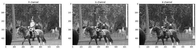
We will further divide the above image into RGB channels to extract colour-dependent features from the image.
# Isolate RGB channels
r = image[:,:,0]
g = image[:,:,1]
b = image[:,:,2]

# Visualize the individual color channels
f, (ax1, ax2, ax3) = plt.subplots(1, 3, figsize=(20,10))
ax1.set_title('R channel')
ax1.imshow(r, cmap='gray')
ax2.set_title('G channel')
ax2.imshow(g, cmap='gray')
ax3.set_title('B channel')
ax3.imshow(b, cmap='gray')
# Isolate RGB channels
r = image[:,:,0]
g = image[:,:,1]
b = image[:,:,2]

# Visualize the individual color channels
f, (ax1, ax2, ax3) = plt.subplots(1, 3, figsize=(20,10))
ax1.set_title('R channel')
ax1.imshow(r)
ax2.set_title('G channel')
ax2.imshow(g)
ax3.set_title('B channel')
ax3.imshow(b)

💡 Visualizing the process
📌 Simple Convolution
In the animation above, there is an image of a pixel 5x5. A kernel, also known as a feature extractor or filter, is the dark component that moves over the image and is 3x3 in size. The 3x3 output is referred to as a feature map or an intermediate image, as it does not have all of the properties of the original image. Convolution is used to create the output, which entails extracting a patch of information from the source data, in this case, the kernel. We can see a reduction in pixels and a loss of information due to the Convolution process.
Note: The above convolution process is happening on a single channel.
As can be seen, there is some information loss, indicating that the kernel is focusing on some pixels more and others less. The kernel, which is the pixel in the centre, is more complicated by the pixel that is getting more focus. Edge pixels, on the other hand, receive less attention from the kernel since they are less complex than other pixels. Because the majority of the information in an image is concentrated in the central pixels.
When working with kernels, keep in mind that the size of the kernel should always be in odd numbers, i.e. 3x3, 5x5, 7x7, because keeping the size of kernels even, would result in a loss of symmetry which would not extract information from the image properly leaving some pixels non-convoluted. However, 1x1 kernel size is mostly used for dimensionality reduction and no information is lost during the convolution process of 1x1 size kernel which is called point-to-point convolution.
import matplotlib.pyplot as plt
import matplotlib.image as mpimg

import cv2
import numpy as np

%matplotlib inline

# Read in the image
image = mpimg.imread('input.jpg')

# Convert to grayscale for filtering
gray = cv2.cvtColor(image, cv2.COLOR_RGB2GRAY)

# Convert to grayscale for filtering
gray = cv2.cvtColor(image, cv2.COLOR_RGB2GRAY)

sobel_y = np.array([[ -1, -2, -1],
                   [ 0, 0, 0],
                   [ 1, 2, 1]])
# vertical edge detection
sobel_x = np.array([[-1, 0, 1],
                   [-2, 0, 2],
                   [-1, 0, 1]])
# filter the image using filter2D(grayscale image, bit-depth, kernel)
filtered_image1 = cv2.filter2D(gray, -1, sobel_x)
filtered_image2 = cv2.filter2D(gray, -1, sobel_y)
f, ax = plt.subplots(1, 2, figsize=(15, 4))
ax[0].set_title('horizontal edge detection')
ax[0].imshow(filtered_image1, cmap='gray')
ax[1].set_title('vertical edge detection')
ax[1].imshow(filtered_image2, cmap='gray')

We have two kernels here, one for horizontal edge detection and the other for vertical edge detection, and we can see that they yield different outputs over the same image. This implies the kernel is crucial in determining the overall pattern of the image as well as how much and what data will be recovered from it.
To understand more about the part of kernels and try different kernels and play with values in the neural networks you can visit this link — Image Kernels
📌 Matrix Calculation
🖼 Matrix Calculation
After all, an image utilised in a neural network goes through some matrix calculation, thus we need some values for the convolution of the image. The Kernel value is set to [[0,1,2],[2,2,0],[0,1,2]] and is multiplied by the values of the pixels captured by the Kernel at the time.
📌 Padding

🖼 Padding Concept
Padding is commonly employed to keep the image’s size consistent with that of the input image. The information is reduced, but the image size is preserved, which is dependent on the network and how we want to train the data. Padding involves manually adding a pixel layer over the output image, i.e. the padding data is manually added by the programmer over the output layer.
📌 Stride

🖼 Stride Concept
The stride notion is typically utilised to bypass pixel convolution and speed up the process. The stride specifies how many pixels the kernel should skip before performing the next calculation. The stride value is 1 by default, however, in the following example, stride=2, which means that after one convolution, the kernel skips two pixels at a time for the next convolution operation.
Stride is a hyperparameter that, when utilised correctly, does not cause the image to lose a lot of information. For example, if there is an image of size 1000x1000 then using a stride of 3 would be beneficial as we won’t be losing much data, whereas using the same stride value over a 60x60 image would result in a heavy loss of information. So the Stride value entirely depends on the size of the image.
📌 Feature Accumulation and Aggregation
🖼 Feature Accumulation
Feature accumulation refers to the process of building feature maps from the convolution process of each channel. We have aggregated or collected three feature maps from three channels of the same image in the example above. Similarly, if there are 11 channels, 11 feature maps will be collected, as will 26, 72, and any other number of channels.
Note: For picture convolution, the same filter or kernel is sent via each channel.
Feature aggregation, on the other hand, is a procedure in which we merge all of the acquired feature maps into a single feature map utilising largely mathematics.

🖼 Feature Aggregation
📌 Max Pooling

🖼 Max Pooling Concept
Max Pooling is a pooling operation that calculates the maximum value for patches of a feature map and uses it to create a down-sampled (pooled) feature map. It is usually used after a convolutional layer. It adds a small amount of translation invariance — meaning translating the image by a small amount does not significantly affect the values of most pooled outputs. We will dive deeper into this in the next part of the blog.
📌 Filter Depth
It’s common to have more than one filter. Different filters pick up different qualities of a patch. For example, one filter might look for a particular colour, while another might look for a kind of object of a specific shape. The amount of filters in a convolutional layer is called the filter depth*.*

a patch is connected to a neurone in the next layer
Convolution Neural Network complete architecture

🖼 Complete Convolution Neural Network Architecture
The CNN architecture’s core premise is as follows. The input data contains a 28x28 picture with padding=1, kernel=3x3, stride=1, and activation function=’Relu’ attributes. This resulted in 32 feature maps, implying that it is convoluted across 32 channels, and the layer has padding=1, implying that the output keeps the original image size of 28x28. The information is engulfed into a smaller matrix with the same channels and feature maps, i.e. 32, and the size is decreased to 14x14 in the following layer, where max pooling is used to reduce dimensionality. The third layer uses the same convolution method as the second, while the fourth layer uses the max-pooling method. By now we have collected enough features from the image and the data is ready to roll into the fully connected neural networks.
From the fourth layer, there are 3136 features extracted and flatten and are used as the inputs of the neural network which are connected to 128 neurons in the next layer and the same 128 neurons are connected to another 10 neurons or features in the last layer, this way producing the required output.

🖼 Features extracted by Kernel
To understand more about the feature extraction process, you can check out this blog — Convolutions: Image Convolutions Examples.
💡 Key points
CNN are a category of Neural Networks that have proven very effective in areas such as image recognition and classification which are comprised of one or more convolutional layers followed by one or more fully connected layers as in a standard multilayer neural network.
The filter or the kernel looks at small pieces, or patches, of the image. These patches are the same size as the filter.
Padding is generally used for retaining the size of the image as the same as that of the input image where information reduction is still happening.
The stride concept is used to skip pixel convolution and to fasten the process. Stride is basically how many pixels the kernel should skip for his next calculation.
When we are creating feature maps from the convolution process out of every channel that process is called feature accumulation, and encapsulating all those features into one single feature map is called feature aggregation.
Max Pooling is a pooling operation that calculates the maximum value for patches of a feature map and uses it to create a down-sampled (pooled) feature map.
We will discuss more about Convolutional Neural Networks, Max Pooling and CNN architecture, in the upcoming blog. Also, we will learn about receptive fields and try to understand their importance in CNN.
Till then keep learning. 👍
Next Blog — Understanding Convolution Neural Networks (Part 2)


