AlexNet Architecture Explained

Master's student @Trinity College Dublin | Loves solving complex problems through intelligent systems | Exploring jobs in tech
The convolutional neural network (CNN) architecture known as AlexNet was created by Alex Krizhevsky, Ilya Sutskever, and Geoffrey Hinton, who served as Krizhevsky’s PhD advisor.
Billionaire investor and entrepreneur Peter Thiel’s favourite contrarian question is
What important truth do very few people agree with you on?
If you would have asked this question to Prof. Geoffrey Hinton in 2010. He would have said, “Convolutional Neural Networks (CNN) have the potential to generate a seismic shift in tackling the problem of picture categorization,”. Researchers in the field at the time would not have given such a remark a second thought. Deep Learning wasn’t cool!
That was the year ImageNet Large Scale Visual Recognition Challenge (ILSVRC) was launched.
He and a few other researchers were proven correct in two years with the publication of the paper “Image Net Classification with Deep Neural Networks” by Alex Krizhevsky, Ilya Sutskever, and Geoffrey E. Hinton. The Richter scale was broken by the earthquake! By obliterating outdated concepts in a single, brilliant motion, the article created a new environment for computer vision.
The study employed CNN to obtain a Top-5 error rate of 15.3 per cent(percentage of not correctly identifying an image’s genuine label among its top 5 guesses). The second-best outcome lagged far behind (26.2 per cent). Deep Learning became popular once more after the dust settled.
Several teams would develop CNN architectures over the following few years that would surpass human-level accuracy. After the original author, Alex Krizhevsky, the architecture utilised in the 2012 study is known as AlexNet.
~ introduction from the blog “Understanding AlexNet” by Sunita Nayak.
🧠 AlexNet Architecture
This was the first architecture that used GPU to boost the training performance. AlexNet consists of 5 convolution layers, 3 max-pooling layers, 2 Normalized layers, 2 fully connected layers and 1 SoftMax layer. Each convolution layer consists of a convolution filter and a non-linear activation function called “ReLU”. The pooling layers are used to perform the max-pooling function and the input size is fixed due to the presence of fully connected layers. The input size is mentioned at most of the places as 224x224x3 but due to some padding which happens it works out to be 227x227x3. Above all this AlexNet has over 60 million parameters.
📌 Key Features:
‘ReLU’ is used as an activation function rather than ‘tanh’
Batch size of 128
SGD Momentum is used as a learning algorithm
Data Augmentation is been carried out like flipping, jittering, cropping, colour normalization, etc.
AlexNet was trained on a GTX 580 GPU with only 3 GB of memory which couldn’t fit the entire network. So the network was split across 2 GPUs, with half of the neurons(feature maps) on each GPU.
💡 Max Pooling
Max Pooling is a feature commonly imbibed into Convolutional Neural Network (CNN) architectures. The main idea behind a pooling layer is to “accumulate” features from maps generated by convolving a filter over an image. Formally, its function is to progressively reduce the spatial size of the representation to reduce the number of parameters and computations in the network. The most common form of pooling is max pooling.

🖼 Max Pooling
Max pooling is done in part to help over-fitting by providing an abstracted form of the representation. As well, it reduces the computational cost by reducing the number of parameters to learn and provides basic translation invariance to the internal representation. Max pooling is done by applying a max filter to (usually) non-overlapping sub-regions of the initial representation.
The authors of AlexNet used pooling windows, sized 3×3 with a stride of 2 between the adjacent windows. Due to this overlapping nature of Max Pool, the top-1 error rate was reduced by 0.4% and the top-5 error rate was reduced by 0.3% respectively. If you compare this to using non-overlapping pooling windows of size 2×2 with a stride of 2, that would give the same output dimensions.
💡 ReLU Non-Linearity
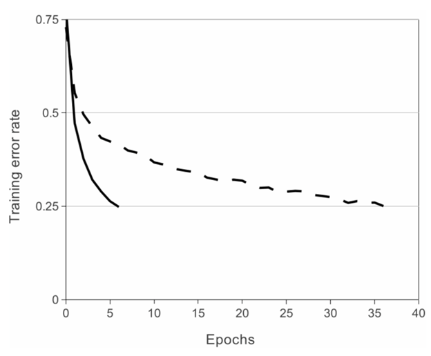
AlexNet demonstrates that saturating activation functions like Tanh or Sigmoid can be used to train deep CNNs much more quickly. The image below demonstrates that AlexNet can achieve a training error rate of 25% with the aid of ReLUs (solid curve). Compared to a network using tanh, this is six times faster (dotted curve). On the CIFAR-10 dataset, this was evaluated.
🖼 ReLU optimization roughly on AlexNet
💡 Data Augmentation
Overfitting can be avoided by showing Neural Net various iterations of the same image. Additionally, it assists in producing more data and compels the Neural Net to memorise the main qualities.
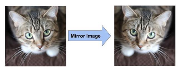
📌 Augmentation by Mirroring
Consider that our training set contains a picture of a cat. A cat can also be seen as its mirror image. This indicates that by just flipping the image above the vertical axis, we may double the size of the training datasets.
🖼 Data Augmentation by Mirroring
📌 Augmentation by Random Cropping of Images
Randomly cropping the original image will also produce additional data that is simply the original data shifted.
For the network’s inputs, the creators of AlexNet selected random crops with dimensions of 227 by 227 from within the 256 by 256 image boundary. They multiplied the size of the data by 2048 using this technique.

🖼 Data Augmentation by Random Cropping
💡 Dropout
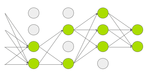
A neuron is removed from the neural network during dropout with a probability of 0.5. A neuron that is dropped does not make any contribution to either forward or backward propagation. As seen in the graphic below, each input is processed by a separate Neural Network design. The acquired weight parameters are therefore more reliable and less prone to overfitting.
📌 AlexNet Summary

Architecture Implementation
📌 Import Libraries and Load the Dataset
For the implementation process, we will be taking a part of the ImageNet dataset by scraping images over the internet using a python library named ‘Beautiful Soup’ and will be passing this dataset on our model to check how is the performance of the AlexNet architecture.
%load_ext tensorboard

import datetime
import numpy as np
import os
import tensorflow as tf
import matplotlib.pyplot as plt
from tqdm import tqdm

from tensorflow.keras import Model
from tensorflow.keras.models import Sequential
from tensorflow.keras.utils import to_categorical
from tensorflow.keras.losses import categorical_crossentropy
from tensorflow.keras.preprocessing.image import ImageDataGenerator
from tensorflow.keras.layers import Dense, Flatten, Conv2D, MaxPooling2D, Dropout

import cv2
import urllib
import requests
import PIL.Image
import numpy as np
from bs4 import BeautifulSoup

#ship synset
page = requests.get("http://www.image-net.org/api/text/imagenet.synset.geturls?wnid=n04194289")
soup = BeautifulSoup(page.content, 'html.parser')
#bicycle synset
bikes_page = requests.get("http://www.image-net.org/api/text/imagenet.synset.geturls?wnid=n02834778")
bikes_soup = BeautifulSoup(bikes_page.content, 'html.parser')

str_soup=str(soup)
split_urls=str_soup.split('\r\n')

bikes_str_soup=str(bikes_soup)
bikes_split_urls=bikes_str_soup.split('\r\n')
📌 Pre-processing
Once we have scraped the images we will be storing the images according to the data labels and we will pre-process the data.
os.mkdir('./content')
os.mkdir('./content/train')
os.mkdir('./content/train/ships')
os.mkdir('./content/train/bikes')
os.mkdir('./content/validation')
os.mkdir('./content/validation/ships')
os.mkdir('./content/validation/bikes')

img_rows, img_cols = 32, 32
input_shape = (img_rows, img_cols, 3)

def url_to_image(url):
    resp = urllib.request.urlopen(url)
    image = np.asarray(bytearray(resp.read()), dtype="uint8")
    image = cv2.imdecode(image, cv2.IMREAD_COLOR)
    return image

n_of_training_images=100
for progress in tqdm(range(n_of_training_images)):
    if not split_urls[progress] == None:
        try:
            I = url_to_image(split_urls[progress])
            if (len(I.shape))==3:
                save_path = './content/train/ships/img'+str(progress)+'.jpg'
                cv2.imwrite(save_path,I)
        except:
            None

for progress in tqdm(range(n_of_training_images)):
    if not bikes_split_urls[progress] == None:
        try:
            I = url_to_image(bikes_split_urls[progress])
            if (len(I.shape))==3:
                save_path = './content/train/bikes/img'+str(progress)+'.jpg'
                cv2.imwrite(save_path,I)
        except:
            None

for progress in tqdm(range(50)):
    if not split_urls[progress] == None:
        try:
            I = url_to_image(split_urls[n_of_training_images+progress])
            if (len(I.shape))==3:
                save_path = './content/validation/ships/img'+str(progress)+'.jpg'
                cv2.imwrite(save_path,I)
        except:
            None


for progress in tqdm(range(50)):
    if not bikes_split_urls[progress] == None:
        try:
            I = url_to_image(bikes_split_urls[n_of_training_images+progress])
            if (len(I.shape))==3:
                save_path = './content/validation/bikes/img'+str(progress)+'.jpg'
                cv2.imwrite(save_path,I)
        except:
            None
📌 Define the Model.
We will be creating the AlexNet Architecture from scratch, although there is a pre-defined function in Keras that will help you to run the AlexNet Architecture.
# AlexNet model
class AlexNet(Sequential):
    def __init__(self, input_shape, num_classes):
        super().__init__()

        self.add(Conv2D(96, kernel_size=(11,11), strides= 4,
                        padding= 'valid', activation= 'relu',
                        input_shape= input_shape,
                        kernel_initializer= 'he_normal'))
        self.add(MaxPooling2D(pool_size=(3,3), strides= (2,2),
                              padding= 'valid', data_format= None))

        self.add(Conv2D(256, kernel_size=(5,5), strides= 1,
                        padding= 'same', activation= 'relu',
                        kernel_initializer= 'he_normal'))
        self.add(MaxPooling2D(pool_size=(3,3), strides= (2,2),
                              padding= 'valid', data_format= None))

        self.add(Conv2D(384, kernel_size=(3,3), strides= 1,
                        padding= 'same', activation= 'relu',
                        kernel_initializer= 'he_normal'))

        self.add(Conv2D(384, kernel_size=(3,3), strides= 1,
                        padding= 'same', activation= 'relu',
                        kernel_initializer= 'he_normal'))

        self.add(Conv2D(256, kernel_size=(3,3), strides= 1,
                        padding= 'same', activation= 'relu',
                        kernel_initializer= 'he_normal'))

        self.add(MaxPooling2D(pool_size=(3,3), strides= (2,2),
                              padding= 'valid', data_format= None))

        self.add(Flatten())
        self.add(Dense(4096, activation= 'relu'))
        self.add(Dense(4096, activation= 'relu'))
        self.add(Dense(1000, activation= 'relu'))
        self.add(Dense(num_classes, activation= 'softmax'))

           self.compile(optimizer= tf.keras.optimizers.Adam(0.001),
                    loss='categorical_crossentropy',
                    metrics=['accuracy'])
📌 Initialize the training parameters
num_classes = 2
model = AlexNet((227, 227, 3), num_classes)

# training parameters
EPOCHS = 100
BATCH_SIZE = 32
image_height = 227
image_width = 227
train_dir = "./content/train"
valid_dir = "./content/validation"
model_dir = "./my_model.h5"

train_datagen = ImageDataGenerator(
                  rescale=1./255,
                  rotation_range=10,
                  width_shift_range=0.1,
                  height_shift_range=0.1,
                  shear_range=0.1,
                  zoom_range=0.1)

train_generator = train_datagen.flow_from_directory(train_dir,
                               target_size=(image_height, image_width),
                               color_mode="rgb",
                               batch_size=BATCH_SIZE,
                               seed=1,
                               shuffle=True,
                               class_mode="categorical")
valid_datagen = ImageDataGenerator(rescale=1.0/255.0)
valid_generator = valid_datagen.flow_from_directory(valid_dir,
                                 target_size=(image_height, image_width),
                                 color_mode="rgb",
                                 batch_size=BATCH_SIZE,
                                 seed=7,
                                 shuffle=True,
                                 class_mode="categorical")
train_num = train_generator.samples
valid_num = valid_generator.samples
📌 Train the model
os.mkdir('./logs')
os.mkdir('./logs/fit')

log_dir="./logs/fit/" + datetime.datetime.now().strftime("%Y%m%d-%H%M%S")
tensorboard_callback = tf.keras.callbacks.TensorBoard(log_dir=log_dir)
callback_list = [tensorboard_callback]

# start training
model.fit(train_generator,
                    epochs=EPOCHS,
                    steps_per_epoch=train_num // BATCH_SIZE,
                    validation_data=valid_generator,
                    validation_steps=valid_num // BATCH_SIZE,
                    callbacks=callback_list,
                    verbose=0)
model.summary()

# save the whole model
model.save(model_dir)

'''
Model: "alex_net"
_________________________________________________________________
Layer (type)                 Output Shape              Param #
=================================================================
conv2d (Conv2D)              (None, 55, 55, 96)        34944
_________________________________________________________________
max_pooling2d (MaxPooling2D) (None, 27, 27, 96)        0
_________________________________________________________________
conv2d_1 (Conv2D)            (None, 27, 27, 256)       614656
_________________________________________________________________
max_pooling2d_1 (MaxPooling2 (None, 13, 13, 256)       0
_________________________________________________________________
conv2d_2 (Conv2D)            (None, 13, 13, 384)       885120
_________________________________________________________________
conv2d_3 (Conv2D)            (None, 13, 13, 384)       1327488
_________________________________________________________________
conv2d_4 (Conv2D)            (None, 13, 13, 256)       884992
_________________________________________________________________
max_pooling2d_2 (MaxPooling2 (None, 6, 6, 256)         0
_________________________________________________________________
flatten (Flatten)            (None, 9216)              0
_________________________________________________________________
dense (Dense)                (None, 4096)              37752832
_________________________________________________________________
dense_1 (Dense)              (None, 4096)              16781312
_________________________________________________________________
dense_2 (Dense)              (None, 1000)              4097000
_________________________________________________________________
dense_3 (Dense)              (None, 2)                 2002
=================================================================
Total params: 62,380,346
Trainable params: 62,380,346
Non-trainable params: 0
_________________________________________________________________
'''
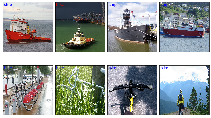
📌 Prediction
class_names = ['bike', 'ship']

x_valid, label_batch  = next(iter(valid_generator))

prediction_values = model.predict_classes(x_valid)

# set up the figure
fig = plt.figure(figsize=(10, 6))
fig.subplots_adjust(left=0, right=1, bottom=0, top=1, hspace=0.05, wspace=0.05)

# plot the images: each image is 227x227 pixels
for i in range(8):
    ax = fig.add_subplot(2, 4, i + 1, xticks=[], yticks=[])
    ax.imshow(x_valid[i,:],cmap=plt.cm.gray_r, interpolation='nearest')

    if prediction_values[i] == np.argmax(label_batch[i]):
        # label the image with the blue text
        ax.text(3, 17, class_names[prediction_values[i]], color='blue', fontsize=14)
    else:
        # label the image with the red text
        ax.text(3, 17, class_names[prediction_values[i]], color='red', fontsize=14)
~ ‘AlexNet Architecture': A Complete Guide by Paras Varshney
Hence, from various blogs, articles and tutorial videos I have tried to present you with a piece of collective information about the AlexNet architecture. I would like to thank all the authors and creators who have done amazing research on this architecture from their side.
And with that, we have completed the AlexNet Architecture, if anyone would like to understand this architecture deeply can check out the paper which was published (The link has been added in the introduction part of this blog). Keep Learning.


